7 Reprojecting geographic data

Prerequisites

• This chapter requires the following packages:

library(sf)
library(terra)
library(dplyr)
library(spData)
library(spDataLarge)

7.1 Introduction

Section 2.4 introduced coordinate reference systems (CRSs), with a focus on the two major types: geographic (‘lon/lat’, with units in degrees longitude and latitude) and projected (typically with units of meters from a datum) coordinate systems. This chapter builds on that knowledge and goes further. It demonstrates how to set and transform geographic data from one CRS to another and, furthermore, highlights specific issues that can arise due to ignoring CRSs that you should be aware of, especially if your data is stored with lon/lat coordinates.

In many projects there is no need to worry about, let alone convert between, different CRSs. Nonetheless, it is important to know if your data is in a projected or geographic coordinate reference system, and the consequences of this for geometry operations. If you know this information, CRSs should just work behind the scenes: people often suddenly need to learn about CRSs when things go wrong. Having a clearly defined CRS that all project data is in, plus understanding how and why to use different CRSs, can ensure that things don’t go wrong. Furthermore, learning about coordinate systems will deepen your knowledge of geographic datasets and how to use them effectively.

This chapter teaches the fundamentals of CRSs, demonstrates the consequences of using different CRSs (including what can go wrong), and how to ‘reproject’ datasets from one coordinate system to another. In the next section we introduce CRSs in R, followed by Section 7.3 which shows how to get and set CRSs associated with spatial objects. Section 7.4 demonstrates the importance of knowing what CRS your data is in with reference to a worked example of creating buffers. We tackle questions of when to reproject and which CRS to use in Section 7.5 and Section 7.6, respectively. Finally, we cover reprojecting vector and raster objects in sections 7.7 and 7.8 and modifying map projections in Section 7.9.

7.2 Coordinate Reference Systems

Most modern geographic tools that require CRS conversions, including core R-spatial packages and desktop GIS software such as QGIS, interface with PROJ, an open source C++ library that “transforms coordinates from one coordinate reference system (CRS) to another”. CRSs can be described in many ways, including the following:

1. Simple yet potentially ambiguous statements such as “it’s in lon/lat coordinates”
2. Formalized yet now outdated ‘proj4 strings’ (also known as ‘proj-string’) such as +proj=longlat +ellps=WGS84 +datum=WGS84 +no_defs
3. With an identifying ‘authority:code’ text string such as EPSG:4326

Each refers to the same thing: the ‘WGS84’ coordinate system that forms the basis of Global Positioning System (GPS) coordinates and many other datasets. But which one is correct?

The short answer is that the third way to identify CRSs is preferable: EPSG:4326 is understood by sf (and by extension stars) and terra packages covered in this book, plus many other software projects for working with geographic data including QGIS and PROJ. EPSG:4326 is future-proof. Furthermore, although it is machine readable, “EPSG:4326” is short, easy to remember and highly ‘findable’ online (searching for EPSG:4326 yields a dedicated page on the website epsg.io, for example). The more concise identifier 4326 is understood by sf, but we recommend the more explicit AUTHORITY:CODE representation to prevent ambiguity and to provide context.

The longer answer is that none of the three descriptions are sufficient and more detail is needed for unambiguous CRS handling and transformations: due to the complexity of CRSs, it is not possible to capture all relevant information about them in such short text strings. For this reason, the Open Geospatial Consortium (OGC, which also developed the simple features specification that the sf package implements) developed an open standard format for describing CRSs that is called WKT (Well-Known Text). This is detailed in a 100+ page document that “defines the structure and content of a text string implementation of the abstract model for coordinate reference systems described in ISO 19111:2019” (Open Geospatial Consortium 2019). The WKT representation of the WGS84 CRS, which has the identifier EPSG:4326 is as follows:

st_crs("EPSG:4326")
#> Coordinate Reference System:
#>   User input: EPSG:4326 
#>   wkt:
#> GEOGCRS["WGS 84",
#>     ENSEMBLE["World Geodetic System 1984 ensemble",
#>         MEMBER["World Geodetic System 1984 (Transit)"],
#>         MEMBER["World Geodetic System 1984 (G730)"],
#>         MEMBER["World Geodetic System 1984 (G873)"],
#>         MEMBER["World Geodetic System 1984 (G1150)"],
#>         MEMBER["World Geodetic System 1984 (G1674)"],
#>         MEMBER["World Geodetic System 1984 (G1762)"],
#>         MEMBER["World Geodetic System 1984 (G2139)"],
#>         ELLIPSOID["WGS 84",6378137,298.257223563,
#>             LENGTHUNIT["metre",1]],
#>         ENSEMBLEACCURACY[2.0]],
#>     PRIMEM["Greenwich",0,
#>         ANGLEUNIT["degree",0.0174532925199433]],
#>     CS[ellipsoidal,2],
#>         AXIS["geodetic latitude (Lat)",north,
#>             ORDER[1],
#>             ANGLEUNIT["degree",0.0174532925199433]],
#>         AXIS["geodetic longitude (Lon)",east,
#>             ORDER[2],
#>             ANGLEUNIT["degree",0.0174532925199433]],
#>     USAGE[
#>         SCOPE["Horizontal component of 3D system."],
#>         AREA["World."],
#>         BBOX[-90,-180,90,180]],
#>     ID["EPSG",4326]]

The output of the command shows how the CRS identifier (also known as a Spatial Reference Identifier or SRID) works: it is simply a look-up, providing a unique identifier associated with a more complete WKT representation of the CRS. This raises the question: what happens if there is a mismatch between the identifier and the longer WKT representation of a CRS? On this point Open Geospatial Consortium (2019) is clear, the verbose WKT representation takes precedence over the identifier:

Should any attributes or values given in the cited identifier be in conflict with attributes or values given explicitly in the WKT description, the WKT values shall prevail.

The convention of referring to CRSs identifiers in the form AUTHORITY:CODE, which is also used by geographic software written in other languages, allows a wide range of formally defined coordinate systems to be referred to.²⁹ The most commonly used authority in CRS identifiers is EPSG, an acronym for the European Petroleum Survey Group which published a standardized list of CRSs (the EPSG was taken over by the Geomatics Committee of the International Association of Oil & Gas Producers in 2005). Other authorities can be used in CRS identifiers. ESRI:54030, for example, refers to ESRI’s implementation of the Robinson projection, which has the following WKT string (only first 8 lines shown):

st_crs("ESRI:54030")
#> Coordinate Reference System:
#>   User input: ESRI:54030 
#>   wkt:
#> PROJCRS["World_Robinson",
#>     BASEGEOGCRS["WGS 84",
#>         DATUM["World Geodetic System 1984",
#>             ELLIPSOID["WGS 84",6378137,298.257223563,
#>                 LENGTHUNIT["metre",1]]],
....

WKT strings are exhaustive, detailed, and precise, allowing for unambiguous CRSs storage and transformations. They contain all relevant information about any given CRS, including its datum and ellipsoid, prime meridian, projection, and units.³⁰

Recent PROJ versions (6+) still allow use of proj-strings to define coordinate operations, but some proj-string keys (+nadgrids, +towgs84, +k, +init=epsg:) are either no longer supported or are discouraged. Additionally, only three datums (i.e., WGS84, NAD83, and NAD27) can be directly set in proj-string. Longer explanations of the evolution of CRS definitions and the PROJ library can be found in Bivand (2021), Chapter 2 of Pebesma and Bivand (2023b), and a blog post by Floris Vanderhaeghe. Also, as outlined in the PROJ documentation there are different versions of the WKT CRS format including WKT1 and two variants of WKT2, the latter of which (WKT2, 2018 specification) corresponds to the ISO 19111:2019 (Open Geospatial Consortium 2019).

7.3 Querying and setting coordinate systems

Let’s look at how CRSs are stored in R spatial objects and how they can be queried and set. First we will look at getting and setting CRSs in vector geographic data objects, starting with the following example:

vector_filepath = system.file("shapes/world.gpkg", package = "spData")
new_vector = read_sf(vector_filepath)

Our new object, new_vector, is a data frame of class sf that represents countries worldwide (see the help page ?spData::world for details). The CRS can be retrieved with the sf function st_crs().

st_crs(new_vector) # get CRS
#> Coordinate Reference System:
#>   User input: WGS 84 
#>   wkt:
#>   ...

The output is a list containing two main components:

1. User input (in this case WGS 84, a synonym for EPSG:4326 which in this case was taken from the input file), corresponding to CRS identifiers described above
2. wkt, containing the full WKT string with all relevant information about the CRS

The input element is flexible, and depending on the input file or user input, can contain the AUTHORITY:CODE representation (e.g., EPSG:4326), the CRS’s name (e.g., WGS 84), or even the proj-string definition. The wkt element stores the WKT representation, which is used when saving the object to a file or doing any coordinate operations. Above, we can see that the new_vector object has the WGS84 ellipsoid, uses the Greenwich prime meridian, and the latitude and longitude axis order. In this case, we also have some additional elements, such as USAGE explaining the area suitable for the use of this CRS, and ID pointing to the CRS’s identifier: EPSG:4326.

The st_crs function also has one helpful feature – we can retrieve some additional information about the used CRS. For example, try to run:

• st_crs(new_vector)$IsGeographic to check is the CRS is geographic or not
• st_crs(new_vector)$units_gdal to find out the CRS units
• st_crs(new_vector)$srid to extract its ‘SRID’ identifier (when available)
• st_crs(new_vector)$proj4string to extract the proj-string representation

In cases when a coordinate reference system (CRS) is missing or the wrong CRS is set, the st_set_crs() function can be used (in this case the WKT string remains unchanged because the CRS was already set correctly when the file was read-in):

new_vector = st_set_crs(new_vector, "EPSG:4326") # set CRS

Getting and setting CRSs works in a similar way for raster geographic data objects. The crs() function in the terra package accesses CRS information from a SpatRaster object (note the use of the cat() function to print it nicely).

raster_filepath = system.file("raster/srtm.tif", package = "spDataLarge")
my_rast = rast(raster_filepath)
cat(crs(my_rast)) # get CRS
#> GEOGCRS["WGS 84",
#>     DATUM["World Geodetic System 1984",
#>         ELLIPSOID["WGS 84",6378137,298.257223563,
#>             LENGTHUNIT["metre",1]]],
#>     PRIMEM["Greenwich",0,
#>         ANGLEUNIT["degree",0.0174532925199433]],
....

The output is the WKT string representation of CRS. The same function, crs(), can be also used to set a CRS for raster objects.

crs(my_rast) = "EPSG:26912" # set CRS

Here, we can use either the identifier (recommended in most cases) or complete WKT string representation. Alternative methods to set crs include proj-string strings or CRSs extracted from other existing object with crs(), although these approaches may be less future proof.

Importantly, the st_crs() and crs() functions do not alter coordinates’ values or geometries. Their role is only to set a metadata information about the object CRS.

In some cases the CRS of a geographic object is unknown, as is the case in the london dataset created in the code chunk below, building on the example of London introduced in Section 2.2:

london = data.frame(lon = -0.1, lat = 51.5) |> 
  st_as_sf(coords = c("lon", "lat"))
st_is_longlat(london)
#> [1] NA

The output NA shows that sf does not know what the CRS is and is unwilling to guess (NA literally means ‘not available’). Unless a CRS is manually specified or is loaded from a source that has CRS metadata, sf does not make any explicit assumptions about which coordinate systems, other than to say “I don’t know”. This behavior makes sense given the diversity of available CRSs but differs from some approaches, such as the GeoJSON file format specification, which makes the simplifying assumption that all coordinates have a lon/lat CRS: EPSG:4326. Datasets without a specified CRS can cause problems: all geographic coordinates have a coordinate reference system and software can only make good decisions around plotting and geometry operations if it knows what type of CRS it is working with. Thus, again, it is important to always check the CRS of a dataset and to set it if it is missing.

london_geo = st_set_crs(london, "EPSG:4326")
st_is_longlat(london_geo)
#> [1] TRUE

7.4 Geometry operations on projected and unprojected data

Since sf version 1.0.0, R’s ability to work with geographic vector datasets that have lon/lat CRSs has improved substantially, thanks to its integration with the S2 spherical geometry engine introduced in Section 2.2.9. As shown in Figure 7.1, sf uses either GEOS or the S2 depending on the type of CRS and whether S2 has been disabled (it is enabled by default). GEOS is always used for projected data and data with no CRS; for geographic data S2 is used by default but can be disabled with sf::sf_use_s2(FALSE).

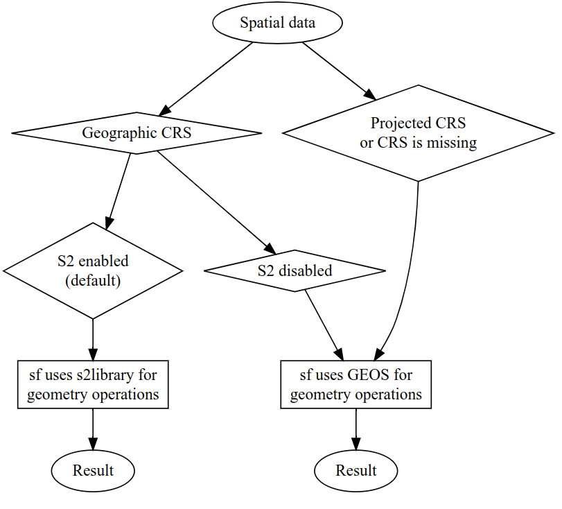
FIGURE 7.1: The behavior of the geometry operations in the sf package depending on the input data’s CRS.

To demonstrate the importance of CRSs, we will create buffer of 100 km around the london object from the previous section. We will also create a deliberately faulty buffer with a ‘distance’ of 1 degree, which is roughly equivalent to 100 km (1 degree is about 111 km at the equator). Before diving into the code, it may be worth skipping briefly ahead to peek at Figure 7.2 to get a visual handle on the outputs that you should be able to reproduce by following the code chunks below.

The first stage is to create three buffers around the london and london_geo objects created above with boundary distances of 1 degree and 100 km (or 100,000 m, which can be expressed as 1e5 in scientific notation) from central London:

london_buff_no_crs = st_buffer(london, dist = 1)   # incorrect: no CRS
london_buff_s2 = st_buffer(london_geo, dist = 100000) # silent use of s2
london_buff_s2_100_cells = st_buffer(london_geo, dist = 100000, max_cells = 100) 

In the first line above, sf assumes that the input is projected and generates a result that has a buffer in units of degrees, which is problematic, as we will see. In the second line, sf silently uses the spherical geometry engine S2, introduced in Chapter 2, to calculate the extent of the buffer using the default value of max_cells = 1000 — set to 100 in line three — the consequences which will become apparent shortly. To highlight the impact of sf’s use of the S2 geometry engine for unprojected (geographic) coordinate systems, we will temporarily disable it with the command sf_use_s2() (which is on, TRUE, by default), in the code chunk below. Like london_buff_no_crs, the new london_geo object is a geographic abomination: it has units of degrees, which makes no sense in the vast majority of cases:

sf::sf_use_s2(FALSE)
#> Spherical geometry (s2) switched off
london_buff_lonlat = st_buffer(london_geo, dist = 1) # incorrect result
#> Warning in st_buffer.sfc(st_geometry(x), dist, nQuadSegs, endCapStyle =
#> endCapStyle, : st_buffer does not correctly buffer longitude/latitude data
#> dist is assumed to be in decimal degrees (arc_degrees).
sf::sf_use_s2(TRUE)
#> Spherical geometry (s2) switched on

The warning message above hints at issues with performing planar geometry operations on lon/lat data. When spherical geometry operations are turned off, with the command sf::sf_use_s2(FALSE), buffers (and other geometric operations) may result in worthless outputs because they use units of latitude and longitude, a poor substitute for proper units of distances such as meters.

The distance between two lines of longitude, called meridians, is around 111 km at the equator (execute geosphere::distGeo(c(0, 0), c(1, 0)) to find the precise distance). This shrinks to zero at the poles. At the latitude of London, for example, meridians are less than 70 km apart (challenge: execute code that verifies this). Lines of latitude, by contrast, are equidistant from each other irrespective of latitude: they are always around 111 km apart, including at the equator and near the poles (see Figures 7.2 to 7.4).

Do not interpret the warning about the geographic (longitude/latitude) CRS as “the CRS should not be set”: it almost always should be! It is better understood as a suggestion to reproject the data onto a projected CRS. This suggestion does not always need to be heeded: performing spatial and geometric operations makes little or no difference in some cases (e.g., spatial subsetting). But for operations involving distances such as buffering, the only way to ensure a good result (without using spherical geometry engines) is to create a projected copy of the data and run the operation on that. This is done in the code chunk below.

london_proj = data.frame(x = 530000, y = 180000) |> 
  st_as_sf(coords = c("x", "y"), crs = "EPSG:27700")

The result is a new object that is identical to london, but created using a suitable CRS (the British National Grid, which has an EPSG code of 27700 in this case) that has units of meters. We can verify that the CRS has changed using st_crs() as follows (some of the output has been replaced by ...,):

st_crs(london_proj)
#> Coordinate Reference System:
#>   User input: EPSG:27700 
#>   wkt:
#> PROJCRS["OSGB36 / British National Grid",
#>     BASEGEOGCRS["OSGB36",
#>         DATUM["Ordnance Survey of Great Britain 1936",
#>             ELLIPSOID["Airy 1830",6377563.396,299.3249646,
#>                 LENGTHUNIT["metre",1]]],
....

Notable components of this CRS description include the EPSG code (EPSG: 27700) and the detailed wkt string (only the first 5 lines of which are shown).³¹ The fact that the units of the CRS, described in the LENGTHUNIT field, are meters (rather than degrees) tells us that this is a projected CRS: st_is_longlat(london_proj) now returns FALSE and geometry operations on london_proj will work without a warning. Buffer operations on the london_proj will use GEOS and results will be returned with proper units of distance. The following line of code creates a buffer around projected data of exactly 100 km:

london_buff_projected = st_buffer(london_proj, 100000)

The geometries of the three london_buff* objects created in the preceding code that have a specified CRS (london_buff_s2, london_buff_lonlat and london_buff_projected) are illustrated in Figure 7.2.

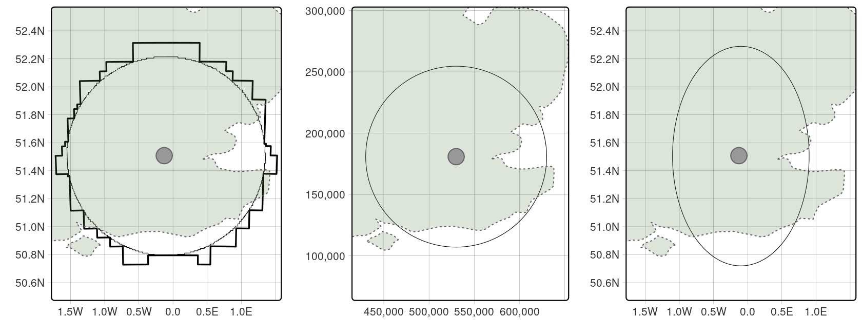
FIGURE 7.2: Buffers around London showing results created with the S2 spherical geometry engine on lon/lat data (left), projected data (middle) and lon/lat data without using spherical geometry (right). The left plot illustrates the result of buffering unprojected data with sf, which calls Google’s S2 spherical geometry engine by default with max cells set to 1000 (thin line). The thick ‘blocky’ line illustrates the result of the same operation with max cells set to 100.

It is clear from Figure 7.2 that buffers based on s2 and properly projected CRSs are not ‘squashed’, meaning that every part of the buffer boundary is equidistant to London. The results that are generated from lon/lat CRSs when s2 is not used, either because the input lacks a CRS or because sf_use_s2() is turned off, are heavily distorted, with the result elongated in the north-south axis, highlighting the dangers of using algorithms that assume projected data on lon/lat inputs (as GEOS does). The results generated using S2 are also distorted, however, although less dramatically. Both buffer boundaries in Figure 7.2 (left) are jagged, although this may only be apparent or relevant for the thick boundary representing a buffer created with the s2 argument max_cells set to 100. The lesson is that results obtained from lon/lat data via S2 will be different from results obtained from using projected data. The difference between S2 derived buffers and GEOS derived buffers on projected data reduce as the value of max_cells increases: the ‘right’ value for this argument may depend on many factors and the default value 1000 is often a reasonable default. When choosing max_cells values, speed of computation should be balanced against resolution of results. In situations where smooth curved boundaries are advantageous, transforming to a projected CRS before buffering (or performing other geometry operations) may be appropriate.

The importance of CRSs (primarily whether they are projected or geographic) and the impacts of sf’s default setting to use S2 for buffers on lon/lat data is clear from the example above. The subsequent sections go into more depth, exploring which CRS to use when projected CRSs are needed and the details of reprojecting vector and raster objects.

7.5 When to reproject?

The previous section showed how to set the CRS manually, with st_set_crs(london, "EPSG:4326"). In real world applications, however, CRSs are usually set automatically when data is read-in. In many projects the main CRS-related task is to transform objects, from one CRS into another. But when should data be transformed? And into which CRS? There are no clear-cut answers to these questions and CRS selection always involves trade-offs (Maling 1992). However, there are some general principles provided in this section that can help you decide.

First it’s worth considering when to transform. In some cases transformation to a geographic CRS is essential, such as when publishing data online with the leaflet package. Another case is when two objects with different CRSs must be compared or combined, as shown when we try to find the distance between two sf objects with different CRSs:

st_distance(london_geo, london_proj)
# > Error: st_crs(x) == st_crs(y) is not TRUE

To make the london and london_proj objects geographically comparable one of them must be transformed into the CRS of the other. But which CRS to use? The answer depends on context: many projects, especially those involving web mapping, require outputs in EPSG:4326, in which case it is worth transforming the projected object. If, however, the project requires planar geometry operations rather than spherical geometry operations engine (e.g., to create buffers with smooth edges), it may be worth transforming data with a geographic CRS into an equivalent object with a projected CRS, such as the British National Grid (EPSG:27700). That is the subject of Section 7.7.

7.6 Which CRS to use?

The question of which CRS is tricky, and there is rarely a ‘right’ answer: “There exist no all-purpose projections, all involve distortion when far from the center of the specified frame” (Bivand, Pebesma, and Gómez-Rubio 2013). Additionally, you should not be attached just to one projection for every task. It is possible to use one projection for some part of the analysis, another projection for a different part, and even some other for visualization. Always try to pick the CRS that serves your goal best!

When selecting geographic CRSs, the answer is often WGS84. It is used not only for web mapping, but also because GPS datasets and thousands of raster and vector datasets are provided in this CRS by default. WGS84 is the most common CRS in the world, so it is worth knowing its EPSG code: 4326.³² This ‘magic number’ can be used to convert objects with unusual projected CRSs into something that is widely understood.

What about when a projected CRS is required? In some cases, it is not something that we are free to decide: “often the choice of projection is made by a public mapping agency” (Bivand, Pebesma, and Gómez-Rubio 2013). This means that when working with local data sources, it is likely preferable to work with the CRS in which the data was provided, to ensure compatibility, even if the official CRS is not the most accurate. The example of London was easy to answer because (a) the British National Grid (with its associated EPSG code 27700) is well known and (b) the original dataset (london) already had that CRS.

A commonly used default is Universal Transverse Mercator (UTM), a set of CRSs that divides the Earth into 60 longitudinal wedges and 20 latitudinal segments. Almost every place on Earth has a UTM code, such as “60H” which refers to northern New Zealand where R was invented. UTM EPSG codes run sequentially from 32601 to 32660 for northern hemisphere locations and from 32701 to 32760 for southern hemisphere locations.

To show how the system works, let’s create a function, lonlat2UTM() to calculate the EPSG code associated with any point on the planet as follows:

lonlat2UTM = function(lonlat) {
  utm = (floor((lonlat[1] + 180) / 6) %% 60) + 1
  if (lonlat[2] > 0) {
    utm + 32600
  } else{
    utm + 32700
  }
}

The following command uses this function to identify the UTM zone and associated EPSG code for Auckland and London:

lonlat2UTM(c(174.7, -36.9))
#> [1] 32760
lonlat2UTM(st_coordinates(london))
#> [1] 32630

The transverse Mercator projection used by UTM CRSs is conformal but distorts areas and distances with increasing severity with distance from the center of the UTM zone. Documentation from the GIS software Manifold therefore suggests restricting the longitudinal extent of projects using UTM zones to 6 degrees from the central meridian (source: manifold.net). Therefore, we recommend using UTM only when your focus is on preserving angles for relatively small area!

Currently, we also have tools helping us to select a proper CRS, which includes the crsuggest package (K. Walker (2022)). The main function in this package, suggest_crs(), takes a spatial object with geographic CRS and returns a list of possible projected CRSs that could be used for the given area.³³ Another helpful tool is a webpage https://jjimenezshaw.github.io/crs-explorer/ that lists CRSs based on selected location and type. Important note: while these tools are helpful in many situations, you need to be aware of the properties of the recommended CRS before you apply it.

In cases where an appropriate CRS is not immediately clear, the choice of CRS should depend on the properties that are most important to preserve in the subsequent maps and analysis. CRSs are either equal-area, equidistant, conformal (with shapes remaining unchanged), or some combination of compromises of those (section 2.4.2). Custom CRSs with local parameters can be created for a region of interest and multiple CRSs can be used in projects when no single CRS suits all tasks. ‘Geodesic calculations’ can provide a fall-back if no CRSs are appropriate (see proj.org/geodesic.html). Regardless of the projected CRS used, the results may not be accurate for geometries covering hundreds of kilometers.

When deciding on a custom CRS, we recommend the following:³⁴

• A Lambert azimuthal equal-area (LAEA) projection for a custom local projection (set latitude and longitude of origin to the center of the study area), which is an equal-area projection at all locations but distorts shapes beyond thousands of kilometers
• Azimuthal equidistant (AEQD) projections for a specifically accurate straight-line distance between a point and the center point of the local projection
• Lambert conformal conic (LCC) projections for regions covering thousands of kilometers, with the cone set to keep distance and area properties reasonable between the secant lines
• Stereographic (STERE) projections for polar regions, but taking care not to rely on area and distance calculations thousands of kilometers from the center

One possible approach to automatically select a projected CRS specific to a local dataset is to create an azimuthal equidistant (AEQD) projection for the center-point of the study area. This involves creating a custom CRS (with no EPSG code) with units of meters based on the center point of a dataset. Note that this approach should be used with caution: no other datasets will be compatible with the custom CRS created and results may not be accurate when used on extensive datasets covering hundreds of kilometers.

The principles outlined in this section apply equally to vector and raster datasets. Some features of CRS transformation however are unique to each geographic data model. We will cover the particularities of vector data transformation in Section 7.7 and those of raster transformation in Section 7.8. Next, Section 7.9, shows how to create custom map projections.

7.7 Reprojecting vector geometries

Chapter 2 demonstrated how vector geometries are made-up of points, and how points form the basis of more complex objects such as lines and polygons. Reprojecting vectors thus consists of transforming the coordinates of these points, which form the vertices of lines and polygons.

Section 7.5 contains an example in which at least one sf object must be transformed into an equivalent object with a different CRS to calculate the distance between two objects.

london2 = st_transform(london_geo, "EPSG:27700")

Now that a transformed version of london has been created, using the sf function st_transform(), the distance between the two representations of London can be found.³⁵ It may come as a surprise that london and london2 are over 2 km apart!³⁶

st_distance(london2, london_proj)
#> Units: [m]
#>      [,1]
#> [1,] 2016

Functions for querying and reprojecting CRSs are demonstrated below with reference to cycle_hire_osm, an sf object from spData that represents ‘docking stations’ where you can hire bicycles in London. The CRS of sf objects can be queried, and as we learned in Section 7.1, set with the function st_crs(). The output is printed as multiple lines of text containing information about the coordinate system:

st_crs(cycle_hire_osm)
#> Coordinate Reference System:
#>   User input: EPSG:4326 
#>   wkt:
#> GEOGCS["WGS 84",
#>     DATUM["WGS_1984",
#>         SPHEROID["WGS 84",6378137,298.257223563,
....

As we saw in Section 7.3, the main CRS components, User input and wkt, are printed as a single entity. The output of st_crs() is in fact a named list of class crs with two elements, single character strings named input and wkt, as shown in the output of the following code chunk:

crs_lnd = st_crs(london_geo)
class(crs_lnd)
#> [1] "crs"
names(crs_lnd)
#> [1] "input" "wkt"

Additional elements can be retrieved with the $ operator, including Name, proj4string and epsg (see ?st_crs and the CRS and tranformation tutorial on the GDAL website for details):

crs_lnd$Name
#> [1] "WGS 84"
crs_lnd$proj4string
#> [1] "+proj=longlat +datum=WGS84 +no_defs"
crs_lnd$epsg
#> [1] 4326

As mentioned in Section 7.2, WKT representation, stored in the $wkt element of the crs_lnd object is the ultimate source of truth. This means that the outputs of the previous code chunk are queries from the wkt representation provided by PROJ, rather than inherent attributes of the object and its CRS.

Both wkt and User Input elements of the CRS are changed when the object’s CRS is transformed. In the code chunk below, we create a new version of cycle_hire_osm with a projected CRS (only the first 4 lines of the CRS output are shown for brevity).

cycle_hire_osm_projected = st_transform(cycle_hire_osm, "EPSG:27700")
st_crs(cycle_hire_osm_projected)
#> Coordinate Reference System:
#>   User input: EPSG:27700 
#>   wkt:
#> PROJCRS["OSGB36 / British National Grid",
#> ...

The resulting object has a new CRS with an EPSG code 27700. But how do we find out more details about this EPSG code, or any code? One option is to search for it online, another is to look at the properties of the CRS object:

crs_lnd_new = st_crs("EPSG:27700")
crs_lnd_new$Name
#> [1] "OSGB36 / British National Grid"
crs_lnd_new$proj4string
#> [1] "+proj=tmerc +lat_0=49 +lon_0=-2 +k=0.9996012717 +x_0=400000
+y_0=-100000 +ellps=airy +units=m +no_defs"
crs_lnd_new$epsg
#> [1] 27700

The result shows that the EPSG code 27700 represents the British National Grid, which could have been found by searching online for “EPSG 27700”.

Printing a spatial object in the console automatically returns its coordinate reference system. To access and modify it explicitly, use the st_crs function, for example, st_crs(cycle_hire_osm).

7.8 Reprojecting raster geometries

The projection concepts described in the previous section apply to rasters. However, there are important differences in reprojection of vectors and rasters: transforming a vector object involves changing the coordinates of every vertex but this does not apply to raster data. Rasters are composed of rectangular cells of the same size (expressed by map units, such as degrees or meters), so it is usually impracticable to transform coordinates of pixels separately. Thus, raster reprojection involves creating a new raster object, often with a different number of columns and rows than the original. The attributes must subsequently be re-estimated, allowing the new pixels to be ‘filled’ with appropriate values. In other words, raster reprojection can be thought of as two separate spatial operations: a vector reprojection of the raster extent to another CRS (Section 7.7), and computation of new pixel values through resampling (Section 5.3.4). Thus in most cases when both raster and vector data are used, it is better to avoid reprojecting rasters and reproject vectors instead.

Reprojection of the regular rasters is also known as warping. Additionally, there is a second similar operation called “transformation”. Instead of resampling all of the values, it leaves all values intact but recomputes new coordinates for every raster cell, changing the grid geometry. For example, it could convert the input raster (a regular grid) into a curvilinear grid. The transformation operation can be performed in R using the stars package.

The raster reprojection process is done with project() from the terra package. Like the st_transform() function demonstrated in the previous section, project() takes a spatial object (a raster dataset in this case) and some CRS representation as the second argument. On a side note – the second argument can also be an existing raster object with a different CRS.

Let’s take a look at two examples of raster transformation: using categorical and continuous data. Land cover data are usually represented by categorical maps. The nlcd.tif file provides information for a small area in Utah, USA obtained from National Land Cover Database 2011 in the NAD83 / UTM zone 12N CRS, as shown in the output of the code chunk below (only first line of output shown).

cat_raster = rast(system.file("raster/nlcd.tif", package = "spDataLarge"))
crs(cat_raster)
#> PROJCRS["NAD83 / UTM zone 12N",
#> ...

In this region, 8 land cover classes were distinguished (a full list of NLCD2011 land cover classes can be found at mrlc.gov):

unique(cat_raster)
#>       levels
#> 1      Water
#> 2  Developed
#> 3     Barren
#> 4     Forest
#> 5  Shrubland
#> 6 Herbaceous
#> 7 Cultivated
#> 8   Wetlands

When reprojecting categorical rasters, the estimated values must be the same as those of the original. This could be done using the nearest neighbor method (near), which sets each new cell value to the value of the nearest cell (center) of the input raster. An example is reprojecting cat_raster to WGS84, a geographic CRS well suited for web mapping. The first step is to obtain the definition of this CRS. The second step is to reproject the raster with the project() function which, in the case of categorical data, uses the nearest neighbor method (near).

cat_raster_wgs84 = project(cat_raster, "EPSG:4326", method = "near")

Many properties of the new object differ from the previous one, including the number of columns and rows (and therefore number of cells), resolution (transformed from meters into degrees), and extent, as illustrated in Table 7.1 (note that the number of categories increases from 8 to 9 because of the addition of NA values, not because a new category has been created — the land cover classes are preserved).

TABLE 7.1: Key attributes in the original (‘cat_raster’) and projected (‘cat_raster_wgs84’) categorical raster datasets.

CRS	nrow	ncol	ncell	resolution	unique_categories
NAD83	1359	1073	1458207	31.5275	8
WGS84	1246	1244	1550024	0.0003	9

Reprojecting numeric rasters (with numeric or in this case integer values) follows an almost identical procedure. This is demonstrated below with srtm.tif in spDataLarge from the Shuttle Radar Topography Mission (SRTM), which represents height in meters above sea level (elevation) with the WGS84 CRS:

con_raster = rast(system.file("raster/srtm.tif", package = "spDataLarge"))
cat(crs(con_raster))
#> GEOGCRS["WGS 84",
#>     DATUM["World Geodetic System 1984",
#>         ELLIPSOID["WGS 84",6378137,298.257223563,
#>             LENGTHUNIT["metre",1]]],
#>     PRIMEM["Greenwich",0,
#>         ANGLEUNIT["degree",0.0174532925199433]],
....

We will reproject this dataset into a projected CRS, but not with the nearest neighbor method which is appropriate for categorical data. Instead, we will use the bilinear method which computes the output cell value based on the four nearest cells in the original raster.³⁷ The values in the projected dataset are the distance-weighted average of the values from these four cells: the closer the input cell is to the center of the output cell, the greater its weight. The following commands create a text string representing WGS 84 / UTM zone 12N, and reproject the raster into this CRS, using the bilinear method (output not shown).

con_raster_ea = project(con_raster, "EPSG:32612", method = "bilinear")
cat(crs(con_raster_ea))

Raster reprojection on numeric variables also leads to changes to values and spatial properties, such as the number of cells, resolution, and extent. These changes are demonstrated in Table 7.2.³⁸

TABLE 7.2: Key attributes in the original (‘con_raster’) and projected (‘con_raster_ea’) continuous raster datasets.

CRS	nrow	ncol	ncell	resolution	mean
WGS84	457	465	212505	0.0008	1843
UTM zone 12N	515	422	217330	83.5334	1842

Of course, the limitations of 2D Earth projections apply as much to vector as to raster data. At best we can comply with two out of three spatial properties (distance, area, direction). Therefore, the task at hand determines which projection to choose. For instance, if we are interested in a density (points per grid cell or inhabitants per grid cell) we should use an equal-area projection (see also Chapter 14).

7.9 Custom map projections

Established CRSs captured by AUTHORITY:CODE identifiers such as EPSG:4326 are well suited for many applications. However, it is desirable to use alternative projections or to create custom CRSs in some cases. Section 7.6 mentioned reasons for using custom CRSs, and provided several possible approaches. Here, we show how to apply these ideas in R.

One is to take an existing WKT definition of a CRS, modify some of its elements, and then use the new definition for reprojecting. This can be done for spatial vectors with st_crs() and st_transform(), and for spatial rasters with crs() and project(), as demonstrated in the following example which transforms the zion object to a custom azimuthal equidistant (AEQD) CRS.

zion = read_sf(system.file("vector/zion.gpkg", package = "spDataLarge"))

Using a custom AEQD CRS requires knowing the coordinates of the center point of a dataset in degrees (geographic CRS). In our case, this information can be extracted by calculating a centroid of the zion area and transforming it into WGS84.

zion_centr = st_centroid(zion)
zion_centr_wgs84 = st_transform(zion_centr, "EPSG:4326")
st_as_text(st_geometry(zion_centr_wgs84))
#> [1] "POINT (-113 37.3)"

Next, we can use the newly obtained values to update the WKT definition of the azimuthal equidistant (AEQD) CRS seen below. Notice that we modified just two values below – "Central_Meridian" to the longitude and "Latitude_Of_Origin" to the latitude of our centroid.

my_wkt = 'PROJCS["Custom_AEQD",
 GEOGCS["GCS_WGS_1984",
  DATUM["WGS_1984",
   SPHEROID["WGS_1984",6378137.0,298.257223563]],
  PRIMEM["Greenwich",0.0],
  UNIT["Degree",0.0174532925199433]],
 PROJECTION["Azimuthal_Equidistant"],
 PARAMETER["Central_Meridian",-113.0263],
 PARAMETER["Latitude_Of_Origin",37.29818],
 UNIT["Meter",1.0]]'

This approach’s last step is to transform our original object (zion) to our new custom CRS (zion_aeqd).

zion_aeqd = st_transform(zion, my_wkt)

Custom projections can also be made interactively, for example, using the Projection Wizard web application (Šavrič, Jenny, and Jenny 2016). This website allows you to select a spatial extent of your data and a distortion property, and returns a list of possible projections. The list also contains WKT definitions of the projections that you can copy and use for reprojections. Also, see Open Geospatial Consortium (2019) for details on creating custom CRS definitions with WKT strings.

PROJ strings can also be used to create custom projections, accepting the limitations inherent to projections, especially of geometries covering large geographic areas, mentioned in Section 7.2. Many projections have been developed and can be set with the +proj= element of PROJ strings, with dozens of projects described in detail on the PROJ website alone.

When mapping the world while preserving area relationships, the Mollweide projection, illustrated in Figure 7.3, is a popular and often sensible choice (Jenny et al. 2017). To use this projection, we need to specify it using the proj-string element, "+proj=moll", in the st_transform function:

world_mollweide = st_transform(world, crs = "+proj=moll")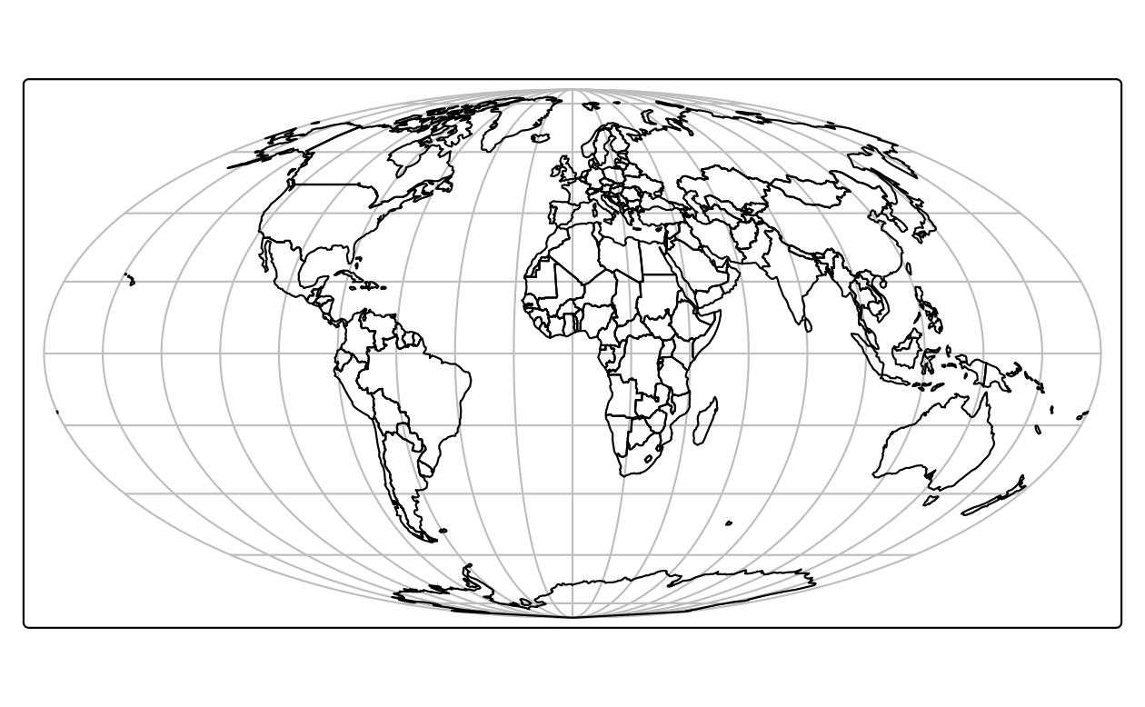

FIGURE 7.3: Mollweide projection of the world.

It is often desirable to minimize distortion for all spatial properties (area, direction, distance) when mapping the world. One of the most popular projections to achieve this is Winkel tripel, illustrated in Figure 7.4.³⁹ The result was created with the following command:

world_wintri = st_transform(world, crs = "+proj=wintri")

FIGURE 7.4: Winkel tripel projection of the world.

Moreover, proj-string parameters can be modified in most CRS definitions, for example the center of the projection can be adjusted using the +lon_0 and +lat_0 parameters. The below code transforms the coordinates to the Lambert azimuthal equal-area projection centered on the longitude and latitude of New York City (Figure 7.5).

world_laea2 = st_transform(world,
                           crs = "+proj=laea +x_0=0 +y_0=0 +lon_0=-74 +lat_0=40")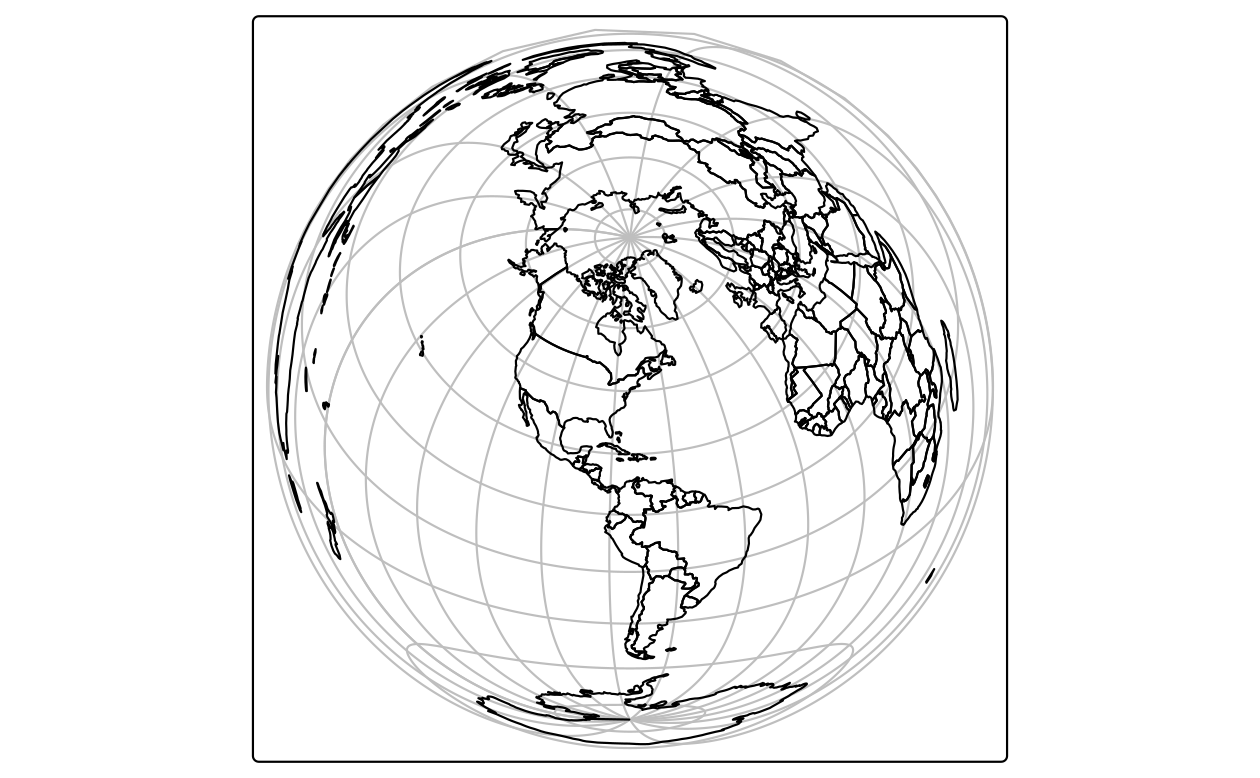

FIGURE 7.5: Lambert azimuthal equal-area projection of the world centered on New York City.

More information on CRS modifications can be found in the Using PROJ documentation.

7.10 Exercises

E1. Create a new object called nz_wgs by transforming nz object into the WGS84 CRS.

• Create an object of class crs for both and use this to query their CRSs.
• With reference to the bounding box of each object, what units does each CRS use?
• Remove the CRS from nz_wgs and plot the result: what is wrong with this map of New Zealand and why?

E2. Transform the world dataset to the transverse Mercator projection ("+proj=tmerc") and plot the result. What has changed and why? Try to transform it back into WGS 84 and plot the new object. Why does the new object differ from the original one?

E3. Transform the continuous raster (con_raster) into NAD83 / UTM zone 12N using the nearest neighbor interpolation method. What has changed? How does it influence the results?

E4. Transform the categorical raster (cat_raster) into WGS 84 using the bilinear interpolation method. What has changed? How does it influence the results?